Basic properties of images and pixels
Overview
Teaching: min
Exercises: minQuestions
Objectives
Understand that an image is composed of pixels.
Understand what pixels and voxels are.
Examine the values and indices of pixels in an image.
Key Points
Spatial calibration
Overview
Teaching: min
Exercises: ImageJ GUIspatial_calibration/exercises/spatial_calibration_imagejgui.md minQuestions
Objectives
Understand that a pixel index is related to a physical coordinate.
Understand that a spatial calibration allows for physical size measurements.
Isotropy
One speaks of isotropic sampling if the pixels have the same extent in all dimensions (2D or 3D).
While microscopy images typically are isotropic in 2D they are typically anisotropic in 3D with coarser sampling in the z-direction.
It is very convenient for image analysis if pixels are isotropic, thus one sometimes resamples the image during image analysis such that they become isotropic.
Key Points
Lookup table
Overview
Teaching: min
Exercises: ImageJ Macro & GUIlut/exercises/configure_luts_imagejmacro.md minQuestions
Objectives
Understand how the numerical values in an image are transformed into colourful images.
Understand what a lookup table (LUT) is and how to adjust it.
Appreciate that choosing the correct LUT is a very serious responsibility when preparing images for a talk or publication.
Lookup tables
Lookup tables do the mapping from a numeric pixel value to a color. This is the main mechanism how we visualise microscopy image data. In case of doubt, it is always a good idea to show the mapping as an inset in the image (or next to the image).
Single color lookup tables
Single color lookup tables are typically configured by chosing one color such as, e.g., grey or green, and choosing a min and max value that determine the brightness of this color depending on the value of the respective pixel in the following way:
brightness( value ) = ( value - min ) / ( max - min )
In this formula, 1 corresponds to the maximal brightness and 0 corresponds to the minimal brightness that, e.g., your computer monitor can produce.
Depending on the values of value, min and max it can be that the formula yields values that are less than 0 or larger than 1. This is handled by assinging a brightness of 0 even if the formula yields values < 0 and assigning a brightness of 1 even if the forumla yield values larger than 1. In such cases one speaks of “clipping”, because one looses (“clips”) information about the pixel value (see below for an example).
Clipping example
min = 20, max = 100, v1 = 100, v2 = 200
brightness( v1 ) = ( 100 - 20 ) / ( 100 - 20 ) = 1
brightness( v2 ) = ( 200 - 20 ) / ( 100 - 20 ) = 2.25
Both pixel values will be painted with the same brightness as a brightness larger than 1 is not possible (see above).
Multi color lookup tables
As the name suggestes multi color lookup tables map pixel gray values to different colors.
For example:
0 -> black
1 -> green
2 -> blue
3 -> ...
Typical use cases for multi color LUTs are images of a high dynamic range (large differences in gray values) and label mask images (where the pixel values encode object IDs).
Sometimes, also multi color LUTs can be configured in terms of a min and max value. The reason is that multi colors LUTs only have a limited amount of colors, e.g. 256 different colors. For instance, if you have an image that contains a pixel with a value of 300 it is not immediately obvious which color it should get; the min and max settings allow you to configure how to map your larger value range into a limited amount of colors.
Key Points
Binarization
Overview
Teaching: min
Exercises: ImageJ GUIbinarization/exercises/binarization_imagejgui.mdImageJ Macrobinarization/exercises/binarization_imagejmacro.mdImageJ Jythonbinarization/exercises/binarization_jython.md minQuestions
Objectives
Describe the relationship between an intensity image and a derived binary image.
Apply a threshold to distinguish foreground and background pixels
Image thresholding
A common algorithm for binarization is thresholding. A threshold value t is chosen, either manually or automatically,
and all pixels with intensities below t are set to 0, whereas pixels with intensities >= t are set to the value for the foreground.
Depending on the software the foreground value can be different (e.g. 1 in MATLAB or 255 in ImageJ).
p_im(x,y) < t -> p_bin(x,y) = 0
p_im(x,y) >= t -> p_bin(x,y) = 1
It is also possible to define an interval of threshold values, i.e. a lower and upper threshold value. Pixels with intensities within this interval belong to the foreground.
Key Points
Connected component labeling
Overview
Teaching: min
Exercises: ImageJ MorpholibJ Macro & GUIconnected_components/exercises/connected_components_imagejmacro.md minQuestions
Objectives
Understand how objects in images are represented as a label mask image.
Apply connected component labeling to a binary image to create a label mask image.
Connectivity
In an image pixels are ordered in a squared configuration. For performing a connected component analysis
it is important to define which pixels are considered direct neighbors of a pixel. This is called connectivity and defines which
pixels are considered connected to each other. Unfortunately, there is not only one way to define connectivity. Depending,
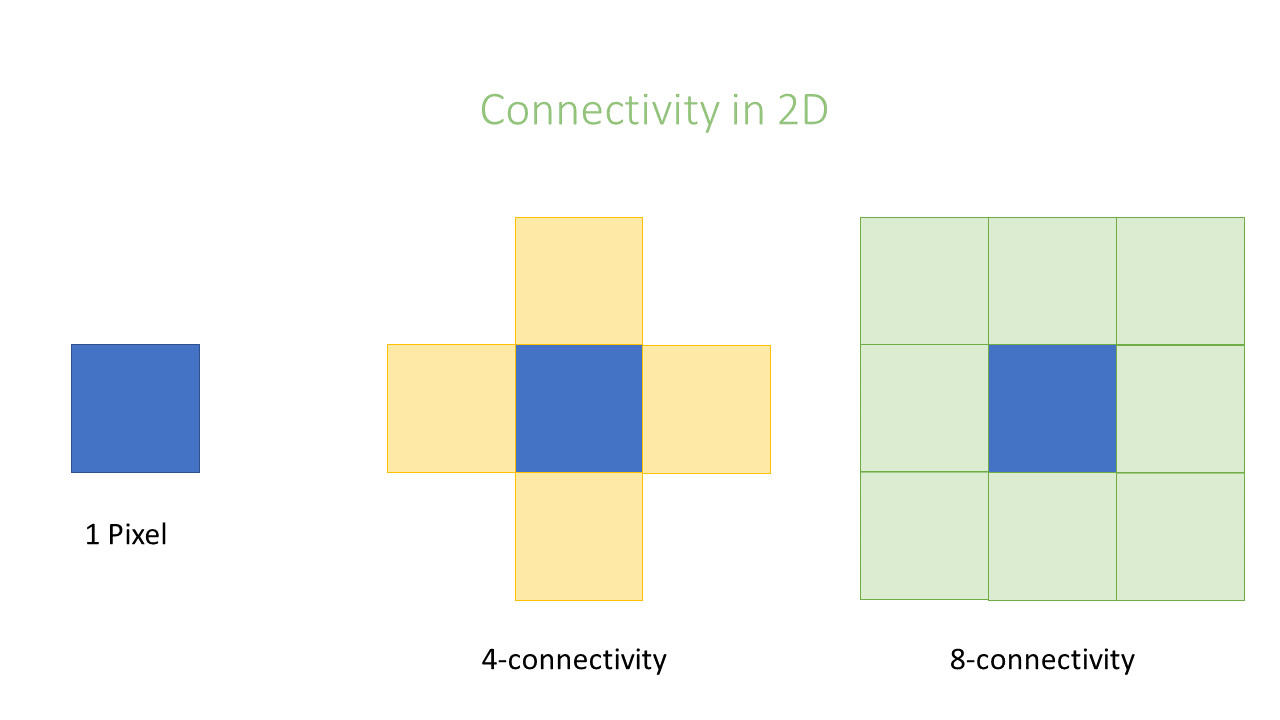
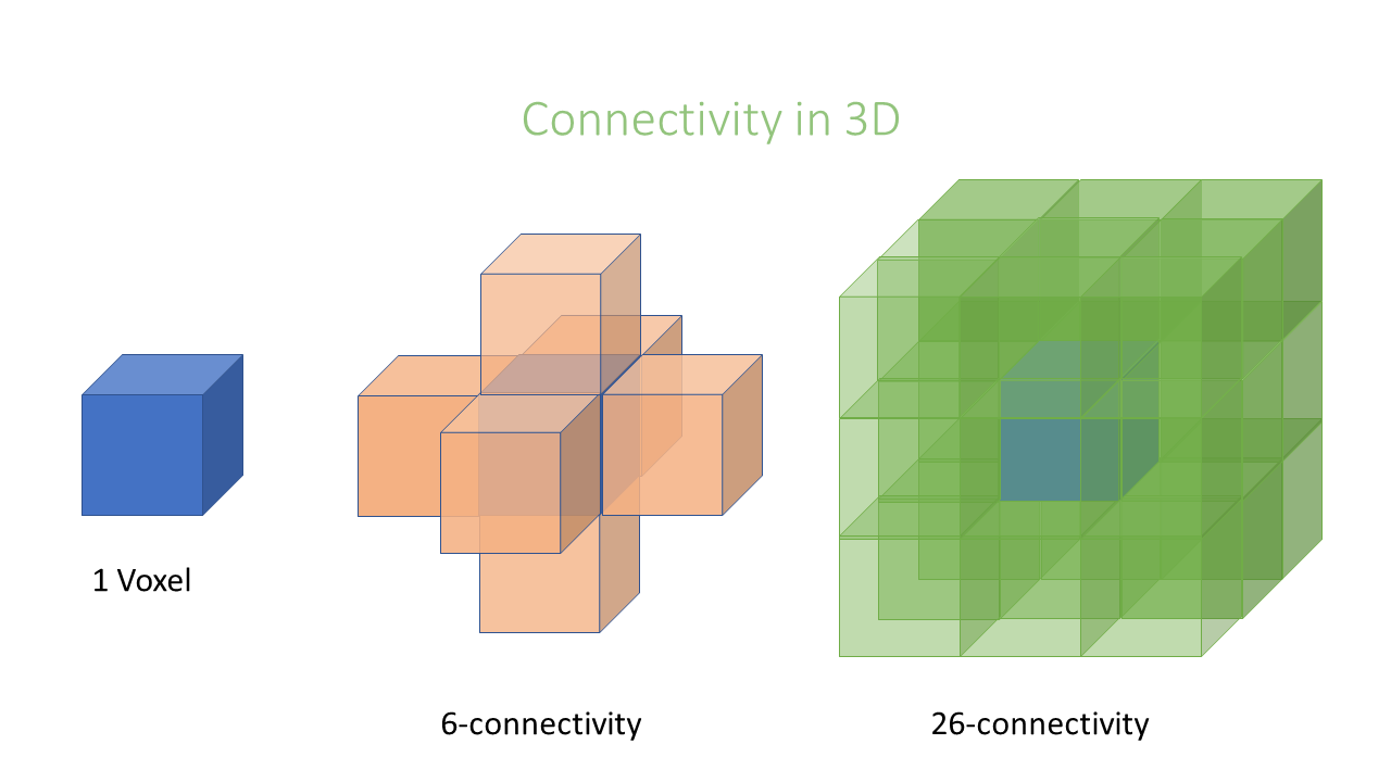
if we consider corner pixels or not we can have in 2D a 4 or 8–connectivity, respectively, in 3D a 6 or 26-connectivity. Which connectivity
value we choose can affect the object size.


Key Points
Data types
Overview
Teaching: min
Exercises: minQuestions
Objectives
Understand that images have a data type which limits the values that the pixels in the image can have.
Understand common data types such as 8-bit and 16-bit unsigned integer.
Image data types
The pixels in an image have a certain data type. The data type limits the values that pixels can take.
For example, unsigned N-bit integer images can represent values from 0 to 2^(N-1), e.g.
- 8-bit unsigned integer: 0 - 255
- 12-bit unsigned integer: 0 - 4095
- 16-bit unsigned integer: 0 - 65535
Intensity clipping (saturation)
If the value of a pixel in an N-bit unsigned integer image is equal to either 0 or 2^(N-1), you cannot know for sure whether you lost information at some point during the image acquisition or image storage. For example, if there is a pixel with the value 255 in an unsigned integer 8-bit image, it may be that the actual intensity “was higher”, e.g. would have corresponded to a gray value of 302. One speaks of “saturation” or “intensity clipping” in such cases. It is important to realise that there can be also clipping at the lower end of the range (some microscopes have an unfortunate “offset” slider that can be set to negative values, which can cause this).
Key Points
Object shape measurements
Overview
Teaching: min
Exercises: ImageJ GUImeasure_shapes/exercises/measure_shapes_imagejgui.md minQuestions
Objectives
Understand shape measurements and their limitations
Perform shape measurements on objects.
Key Points
Workflow - Simple 2D object analysis
Overview
Teaching: min
Exercises: minQuestions
Objectives
Create a simple image analysis workflow.
Understand that bioimage analysis workflows consist of a sequence of image analysis components.
Segment nuclei in a 2D image and measure their shapes and understand the different components (concepts and methods) that are needed to accomplish this task.
Draw a biophysically meaningful conclusion from applying an image analysis workflow to a set of images.
Key Points
Object intensity measurements
Overview
Teaching: min
Exercises: ImageJ Macro & GUImeasure_intensities/exercises/measure_intensities_imagejguimacro.md minQuestions
Objectives
Understand the correct biophysical interpretation of the most common object intensity measurements
Perform object intensity measurements
Background correction
In this module the images that we work are background corrected, meaning that the average intensity in regions without objects is zero. In general this is not the case and, in fact, proper background correction is a super important and very often also quite difficult task in bioimage analysis. There are thus several modules dedicated to background correction for intensity measurements. See below “Learn next” section.
Key points
- Intensity measurements are generally very tricky and most likely the source of many scientific mistakes. Please always consider consulting an bioimage analysis expert!
- Intensity measurements need a background correction. This can be achieved in several ways.
- At least, think carefully about whether the mean or sum intensity is the right readout for your biological question.
- If you publish or present something label your measurement properly, e.g. “Sum Intensity”. Just “Intensity” is not enough!
- Objects based intensity measurements require two input images: the (background corrected) intensity image and a label mask image.
Key Points
Global background correction
Overview
Teaching: min
Exercises: ImageJ Macro & GUIglobal_background_correction/exercises/global_background_correction.md minQuestions
Objectives
Measure the background in an image
Apply image math to subtract a background intensity value from all pixels and understand that the output image should have a floating point data type
Key Points
Neighbourhood filters (introduction)
Overview
Teaching: min
Exercises: ImageJ Macro & GUIfilter_neighbourhood/exercises/filter_mean_imagejmacro.md minQuestions
Objectives
Understand the basic principle of a neighbourhood filter.
Apply a mean filter to an image.
Neighbourhood filters
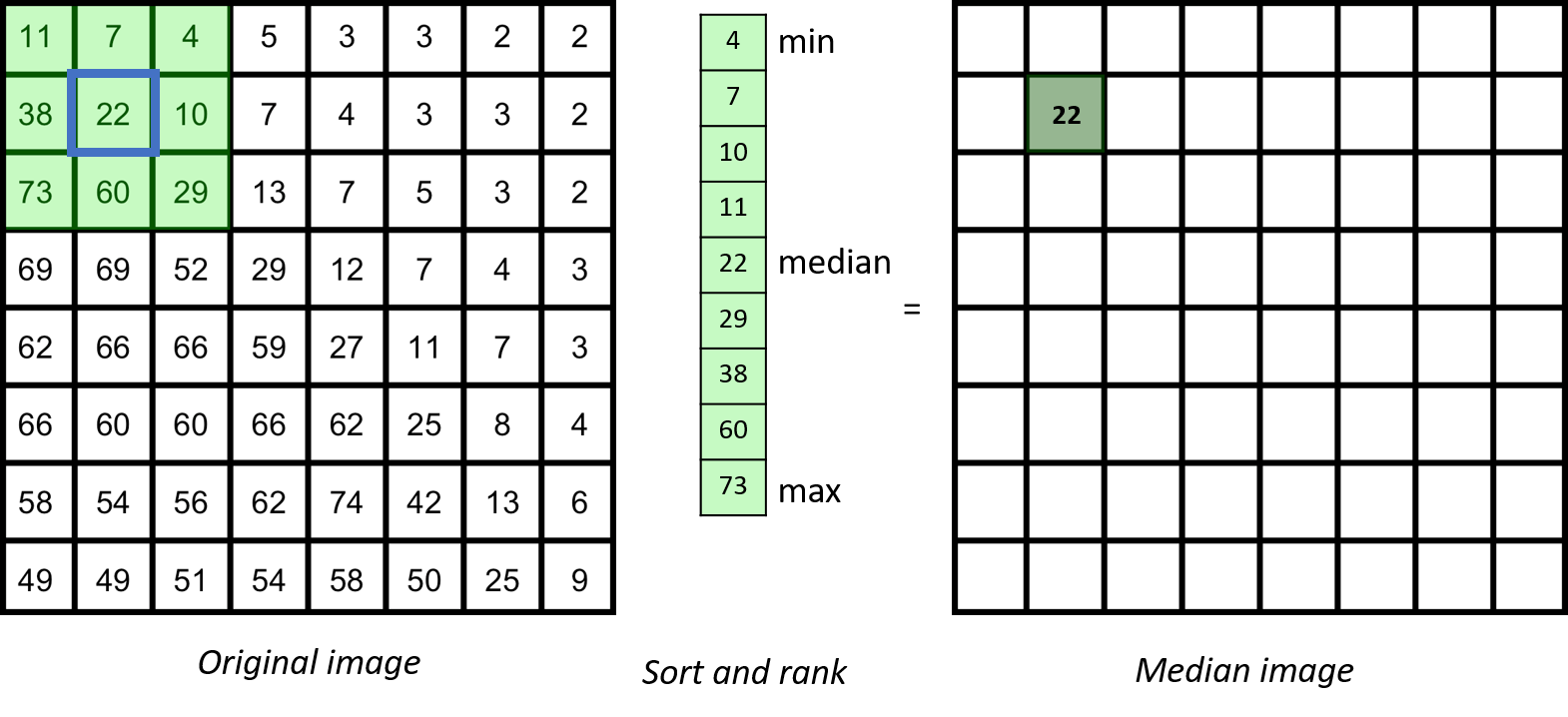
Neighborhood filters comprise two ingredients: a definition of the pixel neighbourhood (size and shape) and a mathematical recipe what to compute on this neighbourhood. The result of this computation will be used to replace the value of the central pixel in the neighbourhood. This procedure can be applied to several (all) pixels of an image to obtain a filtered image. The animation shows a square neighbourhoods (3x3) applied to the inner pixels of the image.
There are really tons of different neighborhood filters, and you can invent a new one!

The neighbourhoods
The neighborhood of a pixel is also called a structuring element and can have various sizes and shapes. Here, we use one of the simplest and most widely used neighbourhoods, namely a circular neighborhood, which is defined by a certain radius. We will explore other shapes of structuring elements in more detail in a dedicated module.
The math
There are really many many ways how to cleverly compute on a pixel neighborhood. For example, one class of computations is called convolutional filters, another is called rank filters. Here, we focus on the relatively simple mean filter, which is the mean filter.
Best practice
As usual, everything depends one the scientific question, but maybe one could say to use a filter that changes the image as little as possible.
Key Points
Median filter
Overview
Teaching: min
Exercises: ImageJ GUImedian_filter/exercises/median_filter_imagejgui.md minQuestions
Objectives
Understand in detail what happens when applying a median filter to an image
Properties of median filter
The median filter is based on ranking the pixels in the neighbourhood

In general, for any neighbourhood filter, if the spatial extend of the neighbourhood is significantly (maybe three-fold) smaller than the smallest spatial length scale that you care about, you are on the safe side.
However, in biology, microscopy images are often containing relevant information down to the level of a single pixel. Thus, you typically have to deal with the fact that filtering may alter your image in a significant way. To judge whether this may affect your scientific conclusions you therefore should study the effect of filters in some detail.
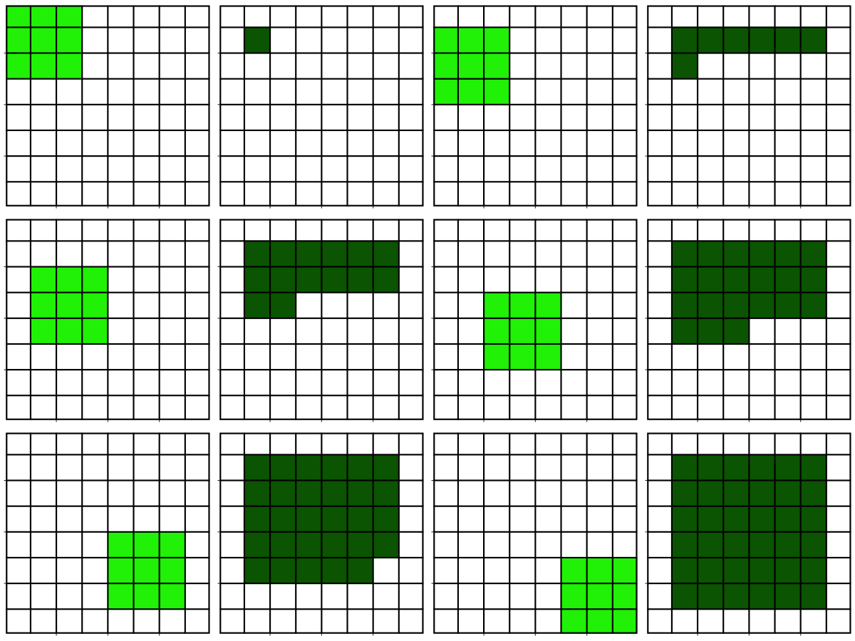
Although a median filter typically is applied to a noisy gray-scale image, understanding its properties is easier when looking at a binary image.
From inspecting the effect of the median filter on above test image, one could say that a median filter
- is edge preserving
- cuts off at convex regions
- fills in at concave regions
- completely removes structures whose shortest axis is smaller than the filter width
Key Points
Local background correction
Overview
Teaching: min
Exercises: ImageJ GUI & Macrolocal_background_correction/exercises/local_background_correction_imagejmacro.md minQuestions
Objectives
Understand how to use image filters for creating a local background image
Use the generated local background image to compute a foreground image
Common filters for creating background images
- Median filter
- “Rolling ball” background
- ImageJ’s “Subtract Background”
- Missing: explanation how it works, exactly
- ImageJ’s “Subtract Background”
- Morphological opening filter
- The result of background subtraction using a grayscale opening is called top-hat filter
Advanced and powerful filters for creating background images
- Morphological opening using reconstruction
- How do the work?
- MATLAB has this option…
imreconstruct - ImageJ MorpholibJ has a Grayscale Attribute Filtering, which seems similar (the same)?
Key Points
Filter objects
Overview
Teaching: min
Exercises: ImageJ Macro & GUIfilter_objects/exercises/filter_objects_imagejmacro_gui.md minQuestions
Objectives
Remove objects from a label mask image.
Key Points
Workflow - 2D noisy object segmentation and filtering
Overview
Teaching: min
Exercises: minQuestions
Objectives
Create an image analysis workflow comprising image denoising and object filtering.
Key Points